
The goal of sewage is to provide a light-weight pipelining interface for data analyses. Rather than construct long scripts with intermiediate datasets or processes, you can construct a single pipeline and run it in a single call.
To download the latest stable release
install.packages("sewage")Or, you can install the development version of sewage from Github:
devtools::install_github("mwhalen18/sewage")Below is an example of how to construct a simple pipeline.
library(sewage)You can use any function as a component in the pipeline, including custom functions you define or import from an external source.
subset_data = function(x) {
  subset(x, cyl == 6)
}
summarizer = function(x) {
  return(summary(x[['disp']]))
}
Currently, there are 3 components ready for use: Nodes,
Splitters, and Joiners. Nodes take one object
as input and return exactly one object. Splitters take in exactly one
object and may return any number of outputs greater than 1.
Joiners take in multiple objects and return 1 object
according to the method you pass to the Joiner (More on
these components below).
pipeline = Pipeline()
pipeline = pipeline |>
  add_node(component = readr::read_csv, name = "Reader", input = "file", show_col_types = FALSE) |>
  add_node(component = Splitter(), name = "Splitter", input = "Reader") |>
  add_node(component = subset_data, name = "Subsetter", input = "Splitter.output_2") |>
  add_node(component = summarizer, name = "Summarizer", input = "Splitter.output_1")
pipeline
#> ══ Pipeline ════════════════════════════════════════════════════════════════════
#> 4 node(s):
#> Reader <-- Input: file
#>
#> Splitter <-- Input: Reader
#>
#> Subsetter <-- Input: Splitter.output_2
#>
#> Summarizer <-- Input: Splitter.output_1Note outputs of a Splitter are accessible by specifying the name of
the splitter component (In this case Splitter) suffixed
with the outgoing edge in the format {name}.output_{i}.
The first node in your pipeline should specify the argument that will be passed into the pipeline when we execute it (More on this below).
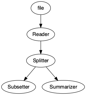
We can easily visualize our pipeline using the draw
method.
draw(pipeline)
Here we execute the pipeline with the run command. It is
important to note that the argument you pass to run should
match the input argument of your first node in your
pipeline. In this case we are passing a file argument in
run and similarly our first node is set to receive a
file argument as input.
You may choose any argument name you like, as long as these two arguments match!
result = run(pipeline, file = 'temp.csv')
#> New names:
#> • `` -> `...1`
print(result)
#> ══ Pipeline [executed] ═════════════════════════════════════════════════════════
#> 4 node(s):
#>  Reader <-- Input: file
#>
#>  Splitter <-- Input: Reader
#>
#>  Subsetter <-- Input: Splitter.output_2
#>
#>  Summarizer <-- Input: Splitter.output_1
#>
#>
#> 2 output(s):
#>  Subsetter
#>
#>  Summarizer
We can now access the results of our terminating nodes. A terminating
node is any node that is not specified as input. By default when the
pipeline is run, each node will overwrite the output of its input node.
Therefore any node that is not fed forward to a new node will return
output. In the case of this pipeline, the Subsetter and
Summarizer edges are our terminating nodes. Therefore, we
can access their results in the outputs object of the
pipeline
pull_output(result, "Subsetter")
#> # A tibble: 7 × 12
#>   ...1           mpg   cyl  disp    hp  drat    wt  qsec    vs    am  gear  carb
#>   <chr>        <dbl> <dbl> <dbl> <dbl> <dbl> <dbl> <dbl> <dbl> <dbl> <dbl> <dbl>
#> 1 Mazda RX4     21       6  160    110  3.9   2.62  16.5     0     1     4     4
#> 2 Mazda RX4 W…  21       6  160    110  3.9   2.88  17.0     0     1     4     4
#> 3 Hornet 4 Dr…  21.4     6  258    110  3.08  3.22  19.4     1     0     3     1
#> 4 Valiant       18.1     6  225    105  2.76  3.46  20.2     1     0     3     1
#> 5 Merc 280      19.2     6  168.   123  3.92  3.44  18.3     1     0     4     4
#> 6 Merc 280C     17.8     6  168.   123  3.92  3.44  18.9     1     0     4     4
#> 7 Ferrari Dino 19.7 6 145 175 3.62 2.77 15.5 0 1 5 6pull_output(result, "Summarizer")
#> Min. 1st Qu. Median Mean 3rd Qu. Max.
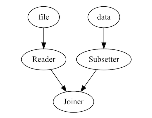
#> 71.1 120.8 196.3 230.7 326.0 472.0It is also possible to pass in multiple entrypoints by specifying the
inputs in your arguments. This allows you to process multiple documents
and bring them together using a Joiner later in your
pipeline.
The Joiner will take multiple inputs and convert them to
a single output in the pipeline according to the function specified.
This component works nicely for dplyr-like joins, but is
not restricted to these methods.
library(dplyr)
pipeline = Pipeline()
pipeline = pipeline |>
  add_node(read.csv, name = "Reader", input = "file") |>
  add_node(subset_data, name = "Subsetter", input = "data") |>
  add_node(Joiner(method = dplyr::bind_rows), name = "Joiner", input = c("Reader", "Subsetter"))
output = run(pipeline, file = "temp.csv", data = mtcars)draw(pipeline)
One of the benefits of {sewage} is that we can pick the pipeline up
at any point using the optional start and halt
options in run. This means we can build an entire data
pipeline, but test small sections. For example, we may want to pass data
down one branch without running the entire pipeline.
pipeline = Pipeline()
pipeline = pipeline |>
  add_node(readr::read_csv, name = "Reader", input = "file", show_col_types = FALSE) |>
  add_node(Splitter(), name = "Splitter", input = "Reader") |>
  add_node(summarizer, name = "Summarizer", input = "Splitter.output_1") |>
  add_node(subset_data, name = "Subsetter", input = "Splitter.output_2") |>
  add_node(func1, name = "Func1", input = "Subsetter") |>
  add_node(func2, name = "Func2", input = "Func1") |>
  add_node(func3, name = "Func3", input = "Func2") |>
  add_node(func4, name = "Func4", input = "Func3") |>
  add_node(func5, name = "Func5", input = "Func4") |>
  add_node(func6, name = "Func6", input = "Summarizer")

result = run(pipeline, start = 'Subsetter', halt = "Func3", Splitter.output_2 = mtcars)
result
#> ══ Pipeline [executed] ═════════════════════════════════════════════════════════
#> 10 node(s):
#>  Reader <-- Input: file
#>
#>  Splitter <-- Input: Reader
#>
#>  Summarizer <-- Input: Splitter.output_1
#>
#>  Subsetter <-- Input: Splitter.output_2
#>
#>  Func1 <-- Input: Subsetter
#>
#>  Func2 <-- Input: Func1
#>
#>  Func3 <-- Input: Func2
#>
#>  Func4 <-- Input: Func3
#>
#>  Func5 <-- Input: Func4
#>
#>  Func6 <-- Input: Summarizer
#>
#>
#> 1 output(s):
#>  Func3
We see that the pipeline has stopped at the “Func3” node. Note we still have to pass the correct input name to the run command just as if it was the first node in the pipeline. Sewage pipelines are executed sequentially in the order you specify them in the pipeline. This means everything after your starting node will be executed and therefore must have an input at runtime. For more information, see the “Building Pipelines” vignette.
Using these three components (Nodes,
Splitters and Joiners) you can construct
complex data pipelines and run them in a single call. By leveraging the
start and halt arguments not only can we
construct large complex data pipelines, but we can isolate components of
the pipeline making data scripts more modular and easier to
maintain.