![]()
![]()
![]()

![]()
rcontroll integrates the individual-based and spatially-explicit TROLL model to simulate forest ecosystem and species dynamics forward in time. rcontroll provides user-friendly functions to set up and analyse simulations with varying community compositions, ecological parameters, and climate conditions.
TROLL is coded in C++ and it typically simulates
hundreds of thousands of individuals over hundreds of years. The
rcontroll R package is a wrapper of TROLL.
rcontroll includes functions that generate inputs for
simulations and run simulations. Finally, it is possible to analyse the
TROLL outputs through tables, figures, and maps taking
advantage of other R visualisation packages. rcontroll also
offers the possibility to generate a virtual LIDAR point cloud that
corresponds to a snapshot of the simulated forest.
As stated above, three types of input data are needed for a typical
TROLL simulation: (i) climate data, (ii) plant functional
traits, (iii) global model parameters. Pre-simulation functions include
global parameters definition (generate_parameters function)
and climate data generation (generate_climate function).
rcontroll also includes default data for species and
climate inputs for a typical French Guiana rainforest site. The purpose
of the generate_climate function with the help of the
corresponding vignette is to create TROLL climate inputs
from ERA5-Land (Muñoz-Sabater et al. 2021), a global climatic reanalysis
dataset that is freely available. The ERA5-Land climate reanalysis is
available at 9 km spatial resolution and hourly temporal resolution
since 1950, and daily or monthly means are available and their
uncertainties reported. Therefore, rcontroll users only
need to input the species-specific trait data to run TROLL
simulations, irrespective of the site. TROLL was originally
developed for tropical and subtropical forests, so certain assumptions
must be critically examined when applying it outside the tropics. The
input files can be used to start a TROLL simulation run
within the rcontroll environment (see below), or saved so
that the TROLL simulation can be started as a command line
tool.
The default option is to run a TROLL simulation using
the troll function of the rcontroll package, which
currently calls version 3.1.7 of TROLL using the Rcpp
package (Eddelbuettel & François 2011). The output is stored in a
trollsim R class. For multiple runs, users can rely on the
stack function, and the output is stored in the
trollstack class. Both trollsim and
trollstack values can be accessed using object attributes
in the form of simple R objects (with @ in R). They consist
of eight simulation attributes: (1) name, (2) path to saved files, (3)
parameters, (4) inputs, (5) log, (6) initial and final state, (7)
ecosystem output metrics, and (8) species output metrics. The initial
and final states are represented by a table with the spatial position,
size and other relevant traits of all trees at the start and end of the
simulation. The ecosystem and species metrics are summaries of ecosystem
processes and states, such as net primary production and aboveground
biomass, and they are documented at species level and aggregated over
the entire stand. Simulations can be saved using a user-defined path
when run and later loaded as a simple simulation
(load_output function) or a stack of simulations
(load_stack function).
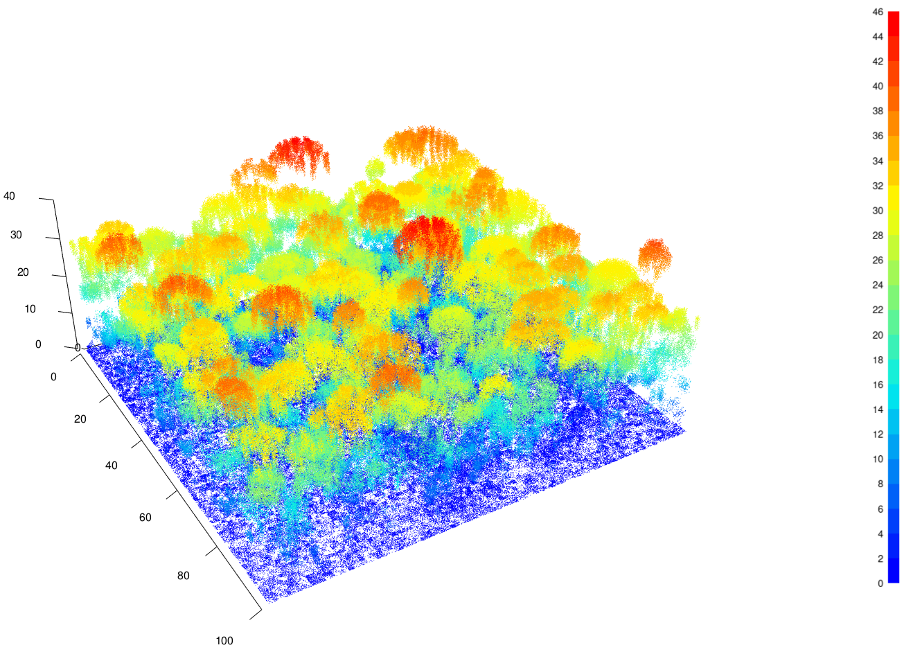
TROLL also has the capacity of generating point clouds
from virtual aerial lidar scannings of simulated forest scenes. Within
each cubic metre voxel of the simulated stand, points are generated
probabilistically, with the probability depending both on the amount of
light reaching the particular voxel and the amount of leaf matter
intercepting light within the voxel. Extinction and interception of
light are based on the Beer-Lambert law, but an effective extinction
factor is used to account for differences between the near-infrared and
visible light. The definition of the lidar parameters
(generate_lidar function) is optional but allows the user
to add a virtual aerial lidar scan for a time step of the
TROLL simulation. When this option is enabled, the cloud of
points from simulated aerial lidar scans are stored as LAS using the R
package lidR (Roussel et al., 2020) as a ninth attribute of
the trollsim and trollstack objects.
rcontroll includes functions to manipulate simulation
outputs. Simulation outputs can be retrieved directly from the
trollsim or trollstackobjects and summarised
or plotted in the R environment with the print,
summary and autoplot functions. The
get_chm function allows users to retrieve canopy height
models from aerial lidar point clouds (Fig. 2). In addition, a
rcontroll function is available to visualise TROLL
simulations as an animated figure (autogif function, Fig.
1).
You can install the latest version of rcontroll from
Github using the devtools
package:
if (!requireNamespace("devtools", quietly = TRUE))
  install.packages("devtools")

devtools::install_github("sylvainschmitt/rcontroll")library(rcontroll)
data("TROLLv3_species")
data("TROLLv3_climatedaytime12")
data("TROLLv3_daytimevar")
sim <- troll(name = "test",
global = generate_parameters(iterperyear = 12, nbiter = 12*1),
species = TROLLv3_species,
climate = TROLLv3_climatedaytime12,
daily = TROLLv3_daytimevar)
autoplot(sim, what = "species",
species = c("Cecropia_obtusa","Dicorynia_guianensis",
"Eperua_grandiflora","Vouacapoua_americana")) +
theme(legend.position = "bottom")