alien is a package dedicated to easily estimate the introduction rates of alien species given first records data. It specializes in addressing the role of sampling on the pattern of discoveries, thus providing better estimates than using Generalized Linear Models which assume perfect immediate detection of newly introduced species.
You can install the CRAN version of the package with:
install.packages("alien")You can install the development version of alien from GitHub with:
# install.packages("devtools")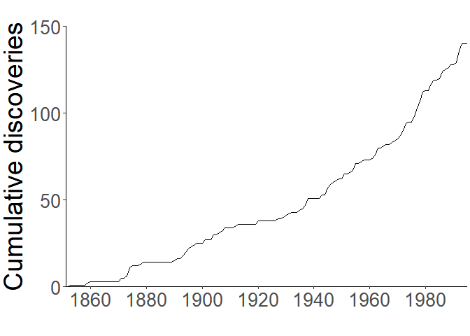
devtools::install_github("hezibu/alien")For the most basic demonstration, let’s look at the data provided in Solow and Costello (2004) which describes discoveries of introduced species in the San Francisco estuary (California, USA) between the years 1850–1995. We’ll plot it in a cumulative form, replicating the plot from Solow and Costello (2004):
library(alien)
library(ggplot2)

data("sfestuary")
years <- seq_along(sfestuary) + 1850

ggplot()+
  aes(x = years, y = cumsum(sfestuary))+
  geom_line() +
  coord_cartesian(ylim = c(0,150))+
  scale_x_continuous(expand = c(0,0), breaks = seq(1860, 1980, 20)) +
  scale_y_continuous(expand = c(0,0), breaks = seq(0, 150, 50)) +
  ylab("Cumulative discoveries") + theme(axis.title.x = element_blank())
As described thoroughly, these discoveries also entail trends in the
probability of detecting new alien species. To estimate the introduction
rate, \({\beta_1}\), from these data,
we will fit the Solow and Costello model using the snc
function. We can use the control argument to pass a list of
options to optim which does the Maximum-Likelihood
Estimation1:
model <- snc(y = sfestuary, control = list(maxit = 1e4))
#> ! no data supplied, using time as independent variable
When only a vector describing discoveries is supplied,
snc warns users that it uses the time as the independent
variable, similar to the original S&C model.
The result is a list containing several objects:
names(model)
#> [1] "records"        "convergence"    "log-likelihood" "coefficients"
#> [5] "type"           "fitted.values"  "predict"
We’ll go over each.
Shows the supplied records data.
model$records
#>   [1] 0 0 1 0 0 0 0 0 1 1 0 0 0 0 0 0 0 0 0 0 2 0 1 5 1 0 0 1 1 0 0 0 0 0 0 0 0
#>  [38] 0 0 1 1 0 2 2 2 1 1 1 0 0 2 0 0 3 0 1 1 2 0 0 0 1 1 0 0 0 0 0 0 2 0 0 0 0
#>  [75] 0 0 1 0 1 1 1 1 0 0 1 1 2 4 0 0 0 0 2 0 4 2 1 1 1 0 3 0 1 1 4 0 1 1 0 0 1
#> [112] 2 4 0 1 1 0 1 1 1 2 3 4 1 0 3 5 4 5 1 0 4 2 0 1 4 1 1 2 0 1 7 4 0 0Did the optimation algorithm converge? This prints out the
convergence code from optim:
model$convergence
#> [1] 0| Code | Meaning/Troubleshooting |
|---|---|
| 0 | Successful convergence |
| 1 | Iteration limit maxit had been reached (increase
maxit using
control = list(maxit = number)) |
| 10 | Degeneracy of the Nelder-Mead simplex |
| 51 | Warning from the "L-BFGS-B"method; Use
debug(snc) and check the optim component
message for further details. |
| 52 | Error from the "L-BFGS-B"method; Use
debug(snc) and check the optim component
message for further details. |
The log-likelihood at the end point of the algorithm (preferably at convergence). Can be used for model selection if needed:
model$`log-likelihood`
#> [1] 118.7776The parameter estimates.
beta0 signifies \({\beta_0}\) - the intercept for \({\mu}\).gamma0 signifies \({\gamma_0}\) - the intercept for \({\Pi}\).gamma2 signifies \({\gamma_2}\) - and will only appear when
the snc argument growth is set to
TRUE (the default).model$coefficients
#> Estimate Std.Err
#> beta0 -1.12739745 1.835403
#> beta1 0.01401579 1.835403
#> gamma0 -185.89484996 15630.676343
#> gamma1 -79.80040427 7235.922667
#> gamma2 76.23985293 6339.859143The fitted \({\lambda_t}\) values of the model. The mean of the Poisson distribution from which the records are assumed to derive.
model$predict
#>          mean      lower_95     higher_95
#> 1   0.3284464  2.464968e-04  4.376407e+02
#> 2   0.3330822  6.848124e-06  1.620061e+04
#> 3   0.3377835  1.902532e-07  5.997150e+05
#> 4   0.3425512  5.285577e-09  2.220028e+07
#> 5   0.3473861  1.468428e-10  8.218113e+08
#> 6   0.3522893  4.079558e-12  3.042185e+10
#> 7   0.3572616  1.133375e-13  1.126158e+12
#> 8   0.3623042  3.148719e-15  4.168817e+13
#> 9   0.3674179  8.747707e-17  1.543215e+15
#> 10  0.3726038  2.430270e-18  5.712682e+16
#> 11  0.3778629  6.751728e-20  2.114724e+18
#> 12  0.3831963  1.875752e-21  7.828296e+19
#> 13  0.3886049  5.211175e-23  2.897883e+21
#> 14  0.3940898  1.447758e-24  1.072740e+23
#> 15  0.3996522  4.022133e-26  3.971074e+24
#> 16  0.4052931  1.117421e-27  1.470014e+26
#> 17  0.4110136  3.104396e-29  5.441708e+27
#> 18  0.4168148  8.624572e-31  2.014414e+29
#> 19  0.4226980  2.396061e-32  7.456970e+30
#> 20  0.4286641  6.656689e-34  2.760425e+32
#> 21  0.4347145  1.849348e-35  1.021856e+34
#> 22  0.4408502  5.137821e-37  3.782711e+35
#> 23  0.4470726  1.427379e-38  1.400286e+37
#> 24  0.4533828  3.965516e-40  5.183587e+38
#> 25  0.4597821  1.101692e-41  1.918863e+40
#> 26  0.4662716  3.060698e-43  7.103257e+41
#> 27  0.4728528  8.503170e-45  2.629488e+43
#> 28  0.4795269  2.362334e-46  9.733852e+44
#> 29  0.4862952  6.562988e-48  3.603283e+46
#> 30  0.4931590  1.823316e-49  1.333865e+48
#> 31  0.5001196  5.065500e-51  4.937709e+49
#> 32  0.5071786  1.407287e-52  1.827844e+51
#> 33  0.5143371  3.909697e-54  6.766323e+52
#> 34  0.5215967  1.086184e-55  2.504761e+54
#> 35  0.5289588  3.017615e-57  9.272138e+55
#> 36  0.5364248  8.383477e-59  3.432365e+57
#> 37  0.5439961  2.329081e-60  1.270595e+59
#> 38  0.5516743  6.470605e-62  4.703495e+60
#> 39  0.5594609  1.797651e-63  1.741142e+62
#> 40  0.5673574  4.994197e-65  6.445370e+63
#> 41  0.5753654  1.387478e-66  2.385951e+65
#> 42  0.5834864  3.854663e-68  8.832325e+66
#> 43  0.5917220  1.070895e-69  3.269555e+68
#> 44  0.6000738  2.975138e-71  1.210326e+70
#> 45  0.6085435  8.265468e-73  4.480390e+71
#> 46  0.6171328  2.296296e-74  1.658553e+73
#> 47  0.6258433  6.379523e-76  6.139641e+74
#> 48  0.6346767  1.772346e-77  2.272776e+76
#> 49  0.6436349  4.923897e-79  8.413374e+77
#> 50  0.6527194  1.367947e-80  3.114467e+79
#> 51  0.6619322  3.800403e-82  1.152915e+81
#> 52  0.6712751  1.055820e-83  4.267868e+82
#> 53  0.6807498  2.933259e-85  1.579882e+84
#> 54  0.6903582  8.149121e-87  5.848415e+85
#> 55  0.7001022  2.263973e-88  2.164969e+87
#> 56  0.7099838  6.289723e-90  8.014295e+88
#> 57  0.7200048  1.747398e-91  2.966736e+90
#> 58  0.7301673  4.854587e-93  1.098228e+92
#> 59  0.7404733  1.348692e-94  4.065427e+93
#> 60  0.7509246  3.746908e-96  1.504942e+95
#> 61  0.7615235  1.040958e-97  5.571002e+96
#> 62  0.7722721  2.891970e-99  2.062277e+98
#> 63  0.7831723 8.034412e-101  7.634147e+99
#> 64  0.7942263 2.232104e-102 2.826013e+101
#> 65  0.8054364 6.201187e-104 1.046135e+103
#> 66  0.8168047 1.722801e-105 3.872588e+104
#> 67  0.8283335 4.786252e-107 1.433557e+106
#> 68  0.8400250 1.329707e-108 5.306748e+107
#> 69  0.8518815 3.694165e-110 1.964455e+109
#> 70  0.8639054 1.026306e-111 7.272030e+110
#> 71  0.8760989 2.851262e-113 2.691964e+112
#> 72  0.8884646 7.921317e-115 9.965127e+113
#> 73  0.9010048 2.200685e-116 3.688896e+115
#> 74  0.9137220 6.113898e-118 1.365558e+117
#> 75  0.9266187 1.698551e-119 5.055029e+118
#> 76  0.9396975 4.718880e-121 1.871273e+120
#> 77  0.9529608 1.310990e-122 6.927089e+121
#> 78  0.9664113 3.642165e-124 2.564274e+123
#> 79  0.9800517 1.011859e-125 9.492443e+124
#> 80  0.9938846 2.811126e-127 3.513918e+126
#> 81  1.0079128 7.809815e-129 1.300784e+128
#> 82  1.0221389 2.169707e-130 4.815249e+129
#> 83  1.0365659 6.027837e-132 1.782512e+131
#> 84  1.0511965 1.674641e-133 6.598511e+132
#> 85  1.0660336 4.652455e-135 2.442640e+134
#> 86  1.0810801 1.292536e-136 9.042180e+135
#> 87  1.0963389 3.590897e-138 3.347239e+137
#> 88  1.1118132 9.976158e-140 1.239083e+139
#> 89  1.1275058 2.771556e-141 4.586843e+140
#> 90  1.1434200 7.699882e-143 1.697960e+142
#> 91  1.1595588 2.139166e-144 6.285518e+143
#> 92  1.1759253 5.942987e-146 2.326777e+145
#> 93  1.1925229 1.651069e-147 8.613275e+146
#> 94  1.2093547 4.586966e-149 3.188467e+148
#> 95  1.2264241 1.274342e-150 1.180308e+150
#> 96  1.2437344 3.540350e-152 4.369272e+151
#> 97  1.2612891 9.835731e-154 1.617419e+153
#> 98  1.2790915 2.732543e-155 5.987372e+154
#> 99  1.2971452 7.591496e-157 2.216409e+156
#> 100 1.3154538 2.109054e-158 8.204714e+157
#> 101 1.3340207 5.859332e-160 3.037225e+159
#> 102 1.3528497 1.627828e-161 1.124322e+161
#> 103 1.3719445 4.522399e-163 4.162021e+162
#> 104 1.3913087 1.256404e-164 1.540699e+164
#> 105 1.4109463 3.490516e-166 5.703368e+165
#> 106 1.4308611 9.697280e-168 2.111276e+167
#> 107 1.4510569 2.694079e-169 7.815533e+168
#> 108 1.4715378 7.484636e-171 2.893158e+170
#> 109 1.4923078 2.079367e-172 1.070991e+172
#> 110 1.5133710 5.776854e-174 3.964600e+173
#> 111 1.5347314 1.604914e-175 1.467618e+175
#> 112 1.5563933 4.458740e-177 5.432836e+176
#> 113 1.5783610 1.238718e-178 2.011130e+178
#> 114 1.6006387 3.441382e-180 7.444812e+179
#> 115 1.6232309 9.560779e-182 2.755925e+181
#> 116 1.6461419 2.656156e-183 1.020190e+183
#> 117 1.6693764 7.379280e-185 3.776544e+184
#> 118 1.6929387 2.050097e-186 1.398003e+186
#> 119 1.7168337 5.695538e-188 5.175135e+187
#> 120 1.7410659 1.582323e-189 1.915734e+189
#> 121 1.7656401 4.395978e-191 7.091676e+190
#> 122 1.7905612 1.221282e-192 2.625201e+192
#> 123 1.8158340 3.392940e-194 9.717982e+193
#> 124 1.8414635 9.426198e-196 3.597408e+195
#> 125 1.8674548 2.618767e-197 1.331690e+197
#> 126 1.8938130 7.275407e-199 4.929659e+198
#> 127 1.9205431 2.021239e-200 1.824864e+200
#> 128 1.9476506 5.615366e-202 6.755291e+201
#> 129 1.9751407 1.560050e-203 2.500677e+203
#> 130 2.0030187 4.334099e-205 9.257021e+204
#> 131 2.0312903 1.204091e-206 3.426769e+206
#> 132 2.0599609 3.345180e-208 1.268523e+208
#> 133 2.0890361 9.293513e-210 4.695826e+209
#> 134 2.1185218 2.581905e-211 1.738304e+211
#> 135 2.1484236 7.172997e-213 6.434861e+212
#> 136 2.1787475 1.992788e-214 2.382061e+214
#> 137 2.2094993 5.536322e-216 8.817925e+215
#> 138 2.2406853 1.538090e-217 3.264224e+217
#> 139 2.2723113 4.273091e-219 1.208352e+219
#> 140 2.3043838 1.187141e-220 4.473085e+220
#> 141 2.3369090 3.298093e-222 1.655849e+222
#> 142 2.3698932 9.162694e-224 6.129631e+223
#> 143 2.4033430 2.545561e-225 2.269070e+225
#> 144 2.4372649 7.072028e-227 8.399657e+226
#> 145 2.4716656 1.964736e-228 3.109390e+228Once we’ve fitted the model, we can use its fit to easily plot \({\lambda_t}\) along with the first records
using the function plot_snc. Users can choose either
annual or cumulative plots. Because the output
is a ggplot object, it can easily be customized
further:
plot_snc(model, cumulative = T) +
  coord_cartesian(ylim = c(0,150))+
  scale_y_continuous(expand = c(0,0), breaks = seq(0, 150, 50)) +
  ylab("Cumulative discoveries") +
  xlab("Years since first record in data")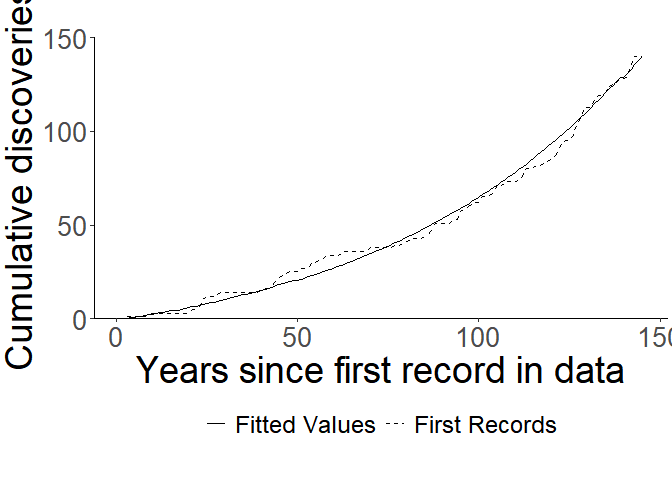
In this case we increase
maxiter so the algorithm will converge↩︎