ILSM:
A package for analyzing the interconnection structure of tripartite
interaction networks (updating)
ILSM is designed to analyze interconnection structures, including
interconnection patterns, centrality, and motifs in tripartite
interaction networks.
Installation
You can install the development version of ILSM from
GitHub:
devtools::install_github("WeichengSun/ILSM")
A
common tripartite interaction network in this package
For clarification, in the following context we refer to a tripartite
network as a two-subnetwork interaction network (Fig. 1a). It is
composed of three sets of nodes (a-nodes, b-nodes, and c-nodes) and two
subnetworks: the P subnetwork, which contains links between a-nodes and
b-nodes, and the Q subnetwork, which contains links between b-nodes and
c-nodes. The b-nodes serve as the shared set of nodes. Connector nodes
are defined as the common nodes of both subnetworks within the b-nodes
(Fig. 1a). No intra-guild interactions are considered unless
specified.
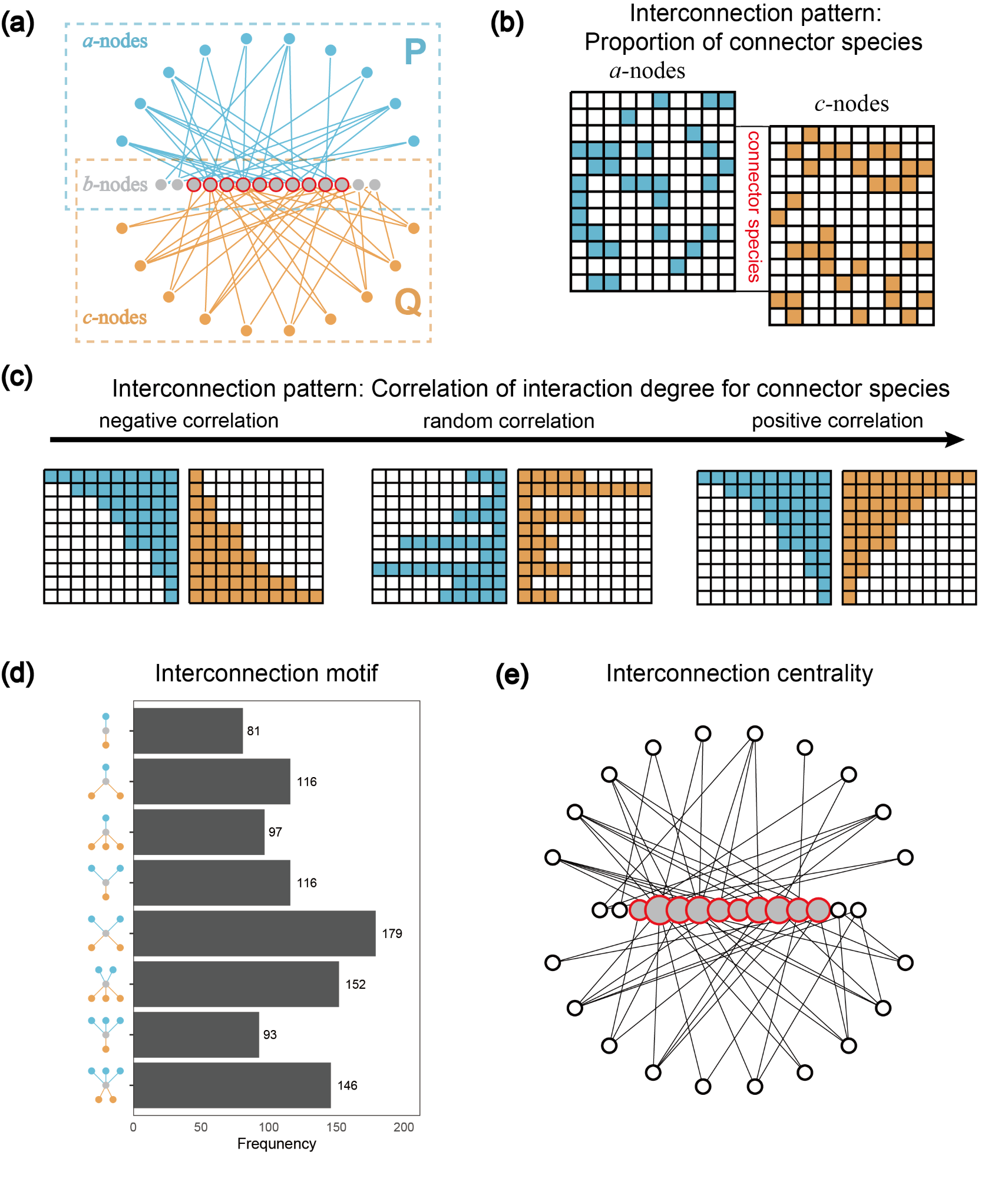 Fig.1. The visualization of an example tripartite interaction network
(a, with three groups of species and two interaction subnetworks) and
interconnection structures for connector species (b-c, two macro-scale
interconnection patterns; d, meso-scale interconnection motif; e,
micro-scale interconnection centrality). In panel a, the connector
species have links from both subnetworks.
Fig.1. The visualization of an example tripartite interaction network
(a, with three groups of species and two interaction subnetworks) and
interconnection structures for connector species (b-c, two macro-scale
interconnection patterns; d, meso-scale interconnection motif; e,
micro-scale interconnection centrality). In panel a, the connector
species have links from both subnetworks.
We provide examples to showcase the functionality of the
ILSM package. First, a worked example demonstrates how to
calculate interconnection patterns, motifs, and centralities (Fig.
1b-c). Second, extensional functions are shown, including null models
and several extra interconnection structures for tripartite networks
with intra-guild interactions.
A
worked example of analyzing interconnection structures
As a worked example, we use a published pollinator–plant–herbivore
(PPH) binary tripartite network (Villa-Galaviz et al. 2021). This PPH
network (PPH_Coltparkmeadow) is a subset of a large
hybrid network that includes plants, flower visitors, leaf miners, and
parasitoids from a long-term nutrient manipulation experiment (Colt Park
Meadows) located at 300 m elevation in Ingleborough National Nature
Reserve, Yorkshire Dales, northern England (54°12′N, 2°21′W). It
contains pollinators, plants, and herbivores, corresponding to
mutualistic interactions in the pollinator–plant subnetwork and
antagonistic interactions in the plant–herbivore subnetwork. Plants are
the shared set of species between the two subnetworks. We also generate
random weights to illustrate the analysis of interconnection structures
in weighted or quantitative tripartite networks.
Interconnection pattern
Interconnection pattern refers to a macro-scale property describing
how connector nodes (species) interconnect two subnetworks. Five
interconnection patterns are supported: proportion of connector nodes
(poc), correlation of interaction degree
(coid), correlation of interaction similarity
(cois), participation coefficient
(pc), and proportion of connector nodes in shared node
hubs (hc).
library(ILSM);library(igraph)
#Load the 'igraph' data
data(PPH_Coltparkmeadow)
#Or read two matrices and transform them to an 'igraph'. .
P_mat<-as.matrix(read.csv("./data/PP.csv",row.names = 1,check.names=FALSE))
Q_mat<-as.matrix(read.csv("./data/HP.csv",row.names = 1,check.names=FALSE))
PPH_Coltparkmeadow<-trigraph_from_mat(P_mat,Q_mat,weighted = F)

#Generating random weights to showcase weighted metrics
E(PPH_Coltparkmeadow)$weight<-runif(length(E(PPH_Coltparkmeadow)),0.1,1.5)

#proportion of connector nodes
poc(PPH_Coltparkmeadow)
poc(P_mat,Q_mat)
#correlation of interaction degree
coid(PPH_Coltparkmeadow)
coid(PPH_Coltparkmeadow,weighted=T)
#correlation of interaction similarity
cois(PPH_Coltparkmeadow)
cois(PPH_Coltparkmeadow,weighted=T)
#participation coefficient
pc(PPH_Coltparkmeadow)
pc(PPH_Coltparkmeadow,weighted=T)
#proportion of connector nodes in shared node hubs
hc(PPH_Coltparkmeadow)
hc(PPH_Coltparkmeadow,weighted=T)
Interconnection motif
Here, we define 48 forms of interconnection motifs (Fig. 2). An
interconnection motif must comprise three sets of connected nodes: the
connector nodes (belonging to the b-nodes), the nodes in one subnetwork
(belonging to the a-nodes in the P subnetwork), and the nodes in the
other subnetwork (belonging to the c-nodes in the Q subnetwork). We
further restrict each motif to contain no more than six nodes and to
have no intra-guild interactions.
The 48 interconnection motifs are provided as igraph objects
through the Multi_motif function in this package.
library(ILSM)
motif_names<-c("M111","M112","M113","M114","M211","M212","M213","M311","M312","M411","M121","M122-1",
       "M122-2","M122-3","M123-1","M123-2","M123-3","M123-4","M123-5","M221-1","M221-2",
       "M221-3","M222-1","M222-2","M222-3","M222-4","M222-5","M222-6","M222-7","M222-8",
       "M222-9","M321-1","M321-2","M321-3","M321-4","M321-5","M131","M132-1","M132-2",
       "M132-3","M132-4","M132-5","M231-1","M231-2","M231-3","M231-4","M231-5","M141")
mr <- par(mfrow=c(6,8),mar=c(1,1,3,1))
IM_res<-Multi_motif("all")
 for(i in 1:48){
     plot(IM_res[[i]],
          vertex.size=30, vertex.label=NA,
          vertex.color="#D0E7ED",main=motif_names[i])
}
par(mr)
The 48 interconnection motifs are named “MABC-i”: M means “motif’,”A”
is the number of a-nodes, “B” is the number of b-nodes, “C” is the
number of c-nodes and “i” is the serial number for the motifs with the
same “ABC”. The interconnection motifs are ordered by the number of
connector nodes (from 1 to 4). The numbers from 1 to 70 in connector
nodes represent the unique roles defined by motifs.
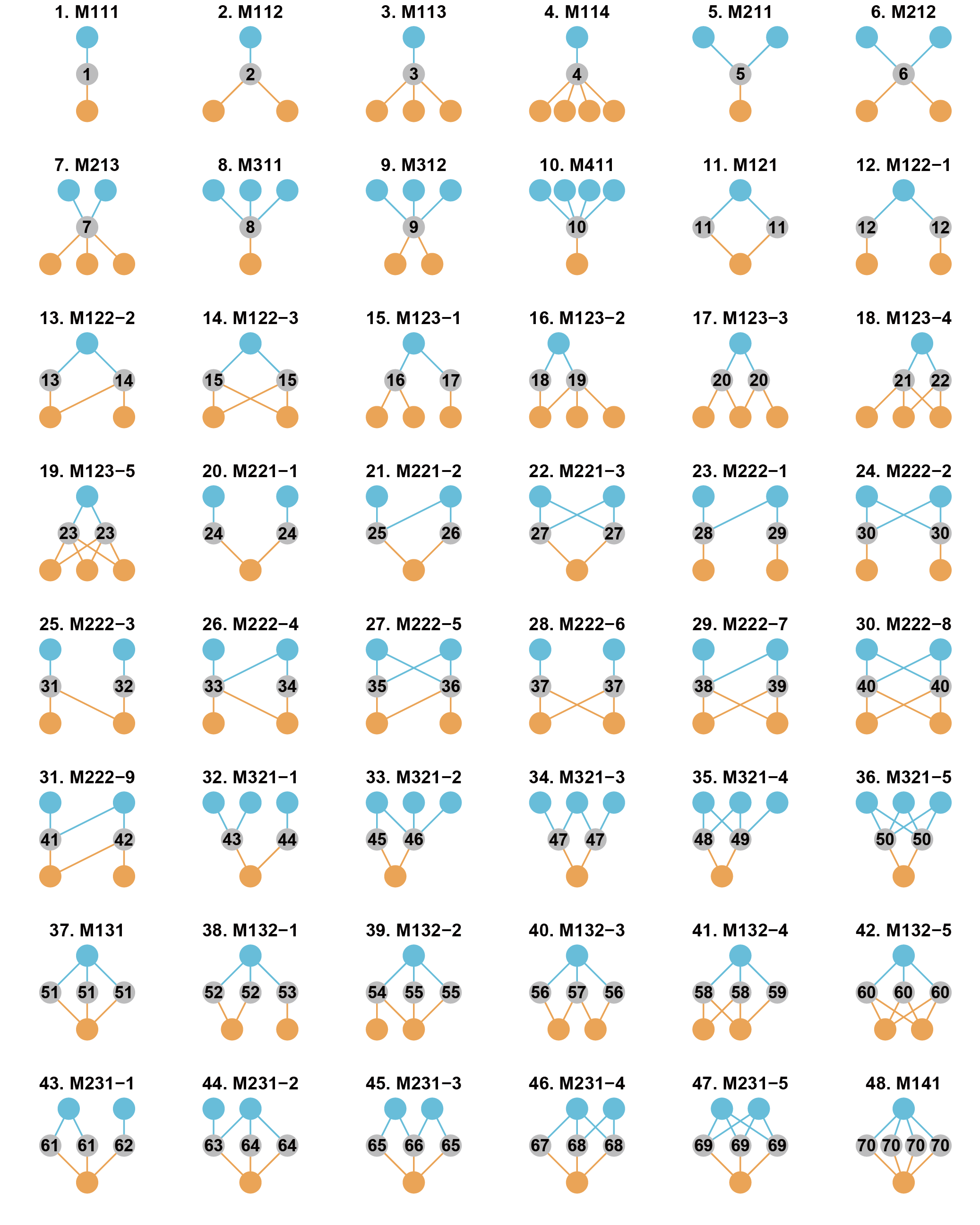 Fig. 2. The 48 forms of interconnection motifs with 3-6 nodes and no
intra-guild interactions. Blue and grey nodes from one subnetwork, and
grey and orange nodes from the other subnetwork. Grey nodes are
connector nodes.
Fig. 2. The 48 forms of interconnection motifs with 3-6 nodes and no
intra-guild interactions. Blue and grey nodes from one subnetwork, and
grey and orange nodes from the other subnetwork. Grey nodes are
connector nodes.
For a tripartite network, the icmotif_count
function returns the counts of each motif, while
icmotif_role provides the counts of motif roles.
icmotif_count(PPH_Coltparkmeadow)
icmotif_role(PPH_Coltparkmeadow)
icmotif_count(PPH_Coltparkmeadow, weighted=T)
icmotif_role(PPH_Coltparkmeadow, weighted=T)
Interconnection centrality
Interconnection centrality measures the importance of connector nodes
in linking two subnetworks within a tripartite network. This differs
from standard centrality measures (e.g., those in igraph),
which treat connector nodes the same as other nodes. The
node_icc provides three interconnection centrality
metrics. For binary networks, interconnection degree centrality for each
connector species is defined as the product of its degree values from
the two subnetworks. Interconnection betweenness centrality is
calculated as the number of shortest paths between a-nodes and c-nodes
that pass through the connector species. Interconnection closeness
centrality is defined as the inverse of the sum of distances from the
connector species to both a-nodes and c-nodes. For weighted networks,
interaction strengths are incorporated into the calculations of weighted
degree, shortest paths, and distances.
node_icc(PPH_Coltparkmeadow)
node_icc(PPH_Coltparkmeadow,weighted=T)
 Fig. 3. The interconnection structures of the example PPH network. (a)
Five interconnection patterns. (b) Three interconnection centrality
indices for eight connector species. (c) The frequencies of 48
interconnection motifs. (d) The frequencies (ln-transformed) of 70 roles
for eight connector species in the interconnection motifs. See codes for
plotting in the vignette.
Fig. 3. The interconnection structures of the example PPH network. (a)
Five interconnection patterns. (b) Three interconnection centrality
indices for eight connector species. (c) The frequencies of 48
interconnection motifs. (d) The frequencies (ln-transformed) of 70 roles
for eight connector species in the interconnection motifs. See codes for
plotting in the vignette.
Extensional analysis
Null models
Null models are commonly used to test the non-randomness of topology
in ecological networks. The tri_null provides two types
of null models. The first type shuffles shared nodes following Sauve et
al. (2016) without altering the subnetwork structures. The second type
shuffles links in one or both subnetworks or layers using algorithms
from the R package vegan (version 2.6-4), applied independently
to one or both subnetworks.
#Testing the significance of CoID, CoIS and interconnection motifs against null models
library(ggplot2);library(pbapply)
set.seed(12)
coid_obs<-coid(PPH_Coltparkmeadow)
cois_obs<-cois(PPH_Coltparkmeadow)
null_net<-vector("list",100)
 i<-1
   while (i<=100) {
      tmp<-tri_null(PPH_Coltparkmeadow,1, null_type = "both_sub",sub_method="r00")[[1]]# try "sauve"
      if(poc(tmp)[2]>=4){# ensuring the simulated networks have at least four connector nodes. This is up to the structure to test. E.g., two few connector nodes led to NA for CoID.
         null_net[[i]]<-tmp;
         i<-i+1
      }}
   coid_null<-pbsapply(null_net,coid)
   cois_null<-pbsapply(null_net,cois)
   icmotif_null<-pbsapply(null_net,function(x){icmotif_count(x)[,2]})# Counts of motifs for null models
   # function to calculate the Z value and P value.
   null_zp<-function(original_value,nullvalues){
      z=(original_value-mean(nullvalues,na.rm=T))/sd(nullvalues,na.rm=T)
      pless <- sum(original_value >= nullvalues, na.rm = TRUE)
      pmore <- sum(original_value <= nullvalues, na.rm = TRUE)
      p<-2 * pmin(pless, pmore)
      p=pmin(1, (p + 1)/(length(nullvalues) + 1))
      c(z=z,p=p)
   }
   # Z and P values
   null_zp(coid_obs,coid_null)# for coid
   null_zp(cois_obs,cois_null)# for cois
   icmotif_null_and_obs<-cbind(icmotif_count(PPH_Coltparkmeadow)[,2],icmotif_null)
   apply( icmotif_null_and_obs,1,function(x){null_zp(x[1],x[-1])})# for motifs
For
tripartite networks with intra-guild interactions
Interconnection
motifs with intra-guild interactions
Although most empirical tripartite interaction networks currently
lack intra-guild interactions, these interactions are increasingly
studied (Garcia-Callejas et al. 2023) and play a crucial role in
community dynamics. Therefore, we also defined interconnection motif
forms that include intra-guild interactions to support potential
meso-scale analyses in tripartite networks. Because incorporating
intra-guild links greatly increases the number of possible motif forms,
we restricted each guild to contain only two nodes, resulting in 107
interconnection motifs. Detailed algorithms: ig_icmotif_count_algorithm,
ig_icmotif_role_algorithm.
 Fig. 4. The 107 forms of interconnection motifs with intra-guild
interactions. Each guild contains only two nodes at most. Blue and grey
nodes from one subnetwork, and grey and orange nodes from the other
subnetwork. Grey nodes are connector nodes.
Fig. 4. The 107 forms of interconnection motifs with intra-guild
interactions. Each guild contains only two nodes at most. Blue and grey
nodes from one subnetwork, and grey and orange nodes from the other
subnetwork. Grey nodes are connector nodes.
For a tripartite network with intra-guild interactions,
ig_icmotif_count returns the counts of each motif,
while ig_icmotif_role returns the counts of motif
roles. Currently, ig_icmotif_role supports role counts only for the 43
roles in the first 35 motifs.
## A toy tripartite network with intra-guild negative interactions, inter-guild mutualistic interactions and inter-guild antagonistic interactions.
set.seed(12)
##4 a-nodes,5 b-nodes, and 3 c-nodes

##intra-guild interaction matrices
mat_aa<-matrix(runif(16,-0.8,-0.2),4,4)
mat_bb<-matrix(runif(25,-0.8,-0.2),5,5)
mat_cc<-matrix(runif(9,-0.8,-0.2),3,3)

##inter-guild interaction matrices between a- and b-nodes.
mat_ab<-mat_ba<-matrix(sample(c(rep(0,8),runif(12,0,0.5))),4,5,byrow=T)# interaction probability = 12/20
mat_ba[mat_ba>0]<-runif(12,0,0.5);mat_ba<-t(mat_ba)

##inter-guild interaction matrices between b- and c-nodes.
mat_cb<-mat_bc<-matrix(sample(c(rep(0,8),runif(7,0,0.5))),3,5,byrow=T)# interaction probability = 7/15
mat_bc[mat_bc>0]<-runif(7,0,0.5);mat_bc<--t(mat_bc)
toy_mat<-rbind(cbind(mat_aa,mat_ab,matrix(0,4,3)),cbind(mat_ba,mat_bb,mat_bc),cbind(matrix(0,3,4),mat_cb,mat_cc))

##set the node names
rownames(toy_mat)<-c(paste0("a",1:4),paste0("b",1:5),paste0("c",1:3));colnames(toy_mat)<-c(paste0("a",1:4),paste0("b",1:5),paste0("c",1:3))
diag(toy_mat)<--1 #assume -1 for diagonal elements

myguilds=c(rep("a",4),rep("b",5),rep("c",3))
ig_icmotif_count(toy_mat,guilds=myguilds)
ig_icmotif_role(toy_mat,guilds=myguilds)
ig_icmotif_count(toy_mat,guilds=myguilds,weighted=T)
ig_icmotif_role(toy_mat,guilds=myguilds, weighted=T)
Degree of diagonal dominance
The ig_ddom calculates the degree of diagonal
dominance for a tripartite network with intra-guild interactions
(Garcia-Callejas et al. 2023).
Species-level
intra-guild and inter-guild interaction overlap
The ig_overlap_guild calculates species-level
intra-guild and inter_guild interaction overlap for a tripartite network
with intra-guild interactions (Garcia-Callejas et al. 2023).
ig_overlap_guild(toy_mat,guilds=myguilds)
License
The code is released under the MIT license (see LICENSE file).
References
Villa-Galaviz, E., et al. 2021. Differential effects of fertilisers
on pollination and parasitoid interaction networks. Journal of Animal
Ecology, 90, 404-414.
Simmons, B. I., Sweering, M. J., Schillinger, M., Dicks, L. V.,
Sutherland, W. J., & Di Clemente, R. 2019. bmotif: A package for
motif analyses of bipartite networks. Methods in Ecology and Evolution,
10(5), 695-701.
Mora, B.B., Cirtwill, A.R. and Stouffer, D.B., 2018. pymfinder: a
tool for the motif analysis of binary and quantitative complex networks.
bioRxiv, 364703.
Domínguez-García, V., & Kéfi, S. 2024. The structure and
robustness of ecological networks with two interaction types. PLOS
Computational Biology, 20(1), e1011770.
Sauve, A. M., Thébault, E., Pocock, M. J., & Fontaine, C. 2016.
How plants connect pollination and herbivory networks and their
contribution to community stability. Ecology, 97(4), 908-917.
Pilosof, S., Porter, M. A., Pascual, M., & Kéfi, S. 2017. The
multilayer nature of ecological networks. Nature Ecology &
Evolution, 1(4), 0101.
Domenico, M. D. 2022. Multilayer Networks: Analysis and
Visualization. Introduction to muxViz with R. . Springer, Cham.
Garcia-Callejas, D., et al. 2023. Non-random interactions within and
across guilds shape the potential to coexist in multi-trophic ecological
communities. Ecology Letters, 26, 831-842.
Citation
Manuscript is being prepared for submission.