BiodiversityR is an R package for statistical analysis
of biodiversity and ecological communities, including species
accumulation curves, diversity indices, Renyi profiles, GLMs for
analysis of species abundance and presence-absence, distance matrices,
Mantel tests, and cluster, constrained and unconstrained ordination
analysis.
The package was initially built to provide a graphical user interface
and different helper functions for the vegan community
ecology package. As documented in a manual on biodiversity and community
ecology analysis, available from this
website and this
link, most analysis pipelines require a community
matrix (typically having sites as rows, species as columns and
abundance values as cell values) and an environmental data
set (typically providing numerical and categorical variables
for the different sites) as inputs. After being launched on CRAN, new
methods from vegan have been integrated in the package as
documented in the ChangeLog file.
A major update of BiodiversityR involved the inclusion
of different methods of ensemble suitability modelling, as described here. Most of
the functions for ensemble suitability modelling were named with a
ensemble.XXXX() naming template.
At the end of 2021, some methods to facilitate plotting results via
ggplot were included in BiodiversityR. These
methods are described in detail in this rpubs series, with some
examples given below.
library(BiodiversityR) # also loads vegan

library(ggplot2)
library(ggforce)
library(concaveman)
library(ggrepel)
library(ggsci)
library(dplyr)
library(pvclust)The data in the examples are data that were used as case study in Data Analysis in Community and Landscape Ecology and also in the Tree Diversity Analysis manual.
Data set dune is a community data set, where variables (columns) typically correspond to different species and data represents abundance of each species. Species names were abbreviated to eight characters, with for example Agrostol representing Agrostis stolonifera.
data(dune)
str(dune)
#> 'data.frame':    20 obs. of  30 variables:
#>  $ Achimill: num  1 3 0 0 2 2 2 0 0 4 ...
#>  $ Agrostol: num  0 0 4 8 0 0 0 4 3 0 ...
#>  $ Airaprae: num  0 0 0 0 0 0 0 0 0 0 ...
#>  $ Alopgeni: num  0 2 7 2 0 0 0 5 3 0 ...
#>  $ Anthodor: num  0 0 0 0 4 3 2 0 0 4 ...
#>  $ Bellpere: num  0 3 2 2 2 0 0 0 0 2 ...
#>  $ Bromhord: num  0 4 0 3 2 0 2 0 0 4 ...
#>  $ Chenalbu: num  0 0 0 0 0 0 0 0 0 0 ...
#>  $ Cirsarve: num  0 0 0 2 0 0 0 0 0 0 ...
#>  $ Comapalu: num  0 0 0 0 0 0 0 0 0 0 ...
#>  $ Eleopalu: num  0 0 0 0 0 0 0 4 0 0 ...
#>  $ Elymrepe: num  4 4 4 4 4 0 0 0 6 0 ...
#>  $ Empenigr: num  0 0 0 0 0 0 0 0 0 0 ...
#>  $ Hyporadi: num  0 0 0 0 0 0 0 0 0 0 ...
#>  $ Juncarti: num  0 0 0 0 0 0 0 4 4 0 ...
#>  $ Juncbufo: num  0 0 0 0 0 0 2 0 4 0 ...
#>  $ Lolipere: num  7 5 6 5 2 6 6 4 2 6 ...
#>  $ Planlanc: num  0 0 0 0 5 5 5 0 0 3 ...
#>  $ Poaprat : num  4 4 5 4 2 3 4 4 4 4 ...
#>  $ Poatriv : num  2 7 6 5 6 4 5 4 5 4 ...
#>  $ Ranuflam: num  0 0 0 0 0 0 0 2 0 0 ...
#>  $ Rumeacet: num  0 0 0 0 5 6 3 0 2 0 ...
#>  $ Sagiproc: num  0 0 0 5 0 0 0 2 2 0 ...
#>  $ Salirepe: num  0 0 0 0 0 0 0 0 0 0 ...
#>  $ Scorautu: num  0 5 2 2 3 3 3 3 2 3 ...
#>  $ Trifprat: num  0 0 0 0 2 5 2 0 0 0 ...
#>  $ Trifrepe: num  0 5 2 1 2 5 2 2 3 6 ...
#>  $ Vicilath: num  0 0 0 0 0 0 0 0 0 1 ...
#>  $ Bracruta: num  0 0 2 2 2 6 2 2 2 2 ...
#>  $ Callcusp: num  0 0 0 0 0 0 0 0 0 0 ...
Data set dune.env is an environmental data set, where variables (columns) correspond to different descriptors (typically continuous and categorical variables) of the sample sites. One of the variables is Management, a categorical variable that describes different management categories, coded as BF (an abbreviation for biological farming), HF (hobby farming), NM (nature conservation management) and SF (standard farming).
data(dune.env)
summary(dune.env)
#>        A1         Moisture Management       Use    Manure
#>  Min.   : 2.800   1:7      BF:3       Hayfield:7   0:6
#>  1st Qu.: 3.500   2:4      HF:5       Haypastu:8   1:3
#>  Median : 4.200   4:2      NM:6       Pasture :5   2:4
#>  Mean   : 4.850   5:7      SF:6                    3:4
#>  3rd Qu.: 5.725                                    4:3
#>  Max.   :11.500
For some plotting methods, it is necessary that the environmental data set is attached:
attach(dune.env)For the examples, we use the constrained ordination method of redundancy analysis.
The ordiplot object is obtained from the result of via function rda. The ordination is done with a community data set that is transformed by the Hellinger method as recommended in this article.
# script generated by the BiodiversityR GUI from the constrained ordination menu
dune.Hellinger <- disttransform(dune, method='hellinger')
Ordination.model1 <- rda(dune.Hellinger ~ Management,
                         data=dune.env,
                         scaling="species")
summary(Ordination.model1)
#>
#> Call:
#> rda(formula = dune.Hellinger ~ Management, data = dune.env, scaling = "species")
#>
#> Partitioning of variance:
#>               Inertia Proportion
#> Total          0.5559     1.0000
#> Constrained    0.1667     0.2999
#> Unconstrained  0.3892     0.7001
#>
#> Eigenvalues, and their contribution to the variance
#>
#> Importance of components:
#>                          RDA1    RDA2    RDA3    PC1     PC2     PC3     PC4
#> Eigenvalue            0.09377 0.05304 0.01988 0.1279 0.05597 0.04351 0.03963
#> Proportion Explained  0.16869 0.09542 0.03575 0.2300 0.10069 0.07827 0.07129
#> Cumulative Proportion 0.16869 0.26411 0.29986 0.5299 0.63054 0.70881 0.78010
#>                           PC5     PC6     PC7     PC8     PC9     PC10     PC11
#> Eigenvalue            0.03080 0.02120 0.01623 0.01374 0.01138 0.009469 0.007651
#> Proportion Explained  0.05541 0.03814 0.02919 0.02471 0.02047 0.017034 0.013764
#> Cumulative Proportion 0.83551 0.87365 0.90284 0.92755 0.94802 0.965056 0.978820
#>                           PC12     PC13     PC14     PC15      PC16
#> Eigenvalue            0.003957 0.003005 0.002485 0.001670 0.0006571
#> Proportion Explained  0.007117 0.005406 0.004470 0.003004 0.0011821
#> Cumulative Proportion 0.985937 0.991344 0.995814 0.998818 1.0000000
#>
#> Accumulated constrained eigenvalues
#> Importance of components:
#>                          RDA1    RDA2    RDA3
#> Eigenvalue            0.09377 0.05304 0.01988
#> Proportion Explained  0.56255 0.31822 0.11923
#> Cumulative Proportion 0.56255 0.88077 1.00000
#>
#> Scaling 2 for species and site scores
#> * Species are scaled proportional to eigenvalues
#> * Sites are unscaled: weighted dispersion equal on all dimensions
#> * General scaling constant of scores:  1.80276
#>
#>
#> Species scores
#>
#>               RDA1      RDA2      RDA3       PC1       PC2       PC3
#> Achimill  0.036568  0.127978  0.016399 -0.188968 -0.070111  0.175399
#> Agrostol -0.003429 -0.270611 -0.018285  0.361207  0.005321 -0.014204
#> Airaprae -0.127487 -0.011618 -0.005281 -0.120126  0.103133  0.060671
#> Alopgeni  0.235229 -0.190348  0.027102  0.163865  0.129547 -0.078901
#> Anthodor -0.085534  0.115742 -0.079991 -0.240230  0.117203  0.201272
#> Bellpere  0.033345  0.041954  0.083723 -0.081623 -0.079661 -0.076104
#> Bromhord  0.093316  0.120369  0.065335 -0.058227 -0.047198  0.043097
#> Chenalbu  0.016343 -0.027339  0.008563  0.006896  0.028380  0.004920
#> Cirsarve  0.019792 -0.033109  0.010370 -0.009773 -0.008401 -0.025099
#> Comapalu -0.110016 -0.010026 -0.004558  0.091463 -0.045993  0.026311
#> Eleopalu -0.160847 -0.069849 -0.041472  0.352544 -0.115164  0.126956
#> Elymrepe  0.173955 -0.047695 -0.002020 -0.108520 -0.206622 -0.115376
#> Empenigr -0.047886 -0.004364 -0.001984 -0.029817  0.061163 -0.018612
#> Hyporadi -0.130851  0.036162  0.047182 -0.127285  0.148136  0.027482
#> Juncarti -0.057086 -0.003074 -0.101556  0.265930 -0.061713 -0.009618
#> Juncbufo  0.102986 -0.052188 -0.062882  0.033316  0.152206 -0.038314
#> Lolipere  0.260211  0.153503  0.052002 -0.192751 -0.234269 -0.146056
#> Planlanc -0.018339  0.192788 -0.064491 -0.222661  0.025888  0.091459
#> Poaprat   0.183546  0.093202  0.019068 -0.196708 -0.136129 -0.115068
#> Poatriv   0.377233 -0.046485 -0.039312 -0.019700 -0.010085  0.010877
#> Ranuflam -0.113470 -0.073249 -0.022781  0.249877 -0.046445  0.073742
#> Rumeacet  0.118187  0.070051 -0.198589 -0.056786  0.065922  0.042193
#> Sagiproc  0.076848 -0.060054  0.017557  0.035039  0.222856 -0.152162
#> Salirepe -0.197203 -0.017971 -0.008170 -0.014209  0.015031 -0.104243
#> Scorautu -0.146131  0.134240  0.015763 -0.059562  0.117768 -0.088453
#> Trifprat  0.061485  0.069094 -0.135080 -0.066713 -0.001921  0.069306
#> Trifrepe  0.010076  0.151446  0.031054  0.039480  0.082043 -0.081712
#> Vicilath -0.014220  0.076123  0.084100 -0.026628  0.009338 -0.057100
#> Bracruta -0.057834  0.021502 -0.054847  0.083143  0.070717 -0.115855
#> Callcusp -0.107307 -0.059711  0.009214  0.169330 -0.068364  0.107835
#>
#>
#> Site scores (weighted sums of species scores)
#>
#>       RDA1    RDA2     RDA3      PC1      PC2       PC3
#> 1   0.5831  0.1826  0.52222 -0.59008 -0.95148 -0.002365
#> 2   0.4752  0.3624  0.90879  0.05773 -0.27927 -0.053465
#> 3   0.5157 -0.3323  0.54177 -0.17847 -0.28527 -0.368932
#> 4   0.4399 -0.3608  0.65164 -0.15066 -0.12951 -0.386916
#> 5   0.2767  0.7135 -0.68027 -0.32785 -0.13648  0.331094
#> 6   0.1630  0.7846 -0.99354 -0.24794  0.06413  0.280023
#> 7   0.3075  0.7908 -0.69144 -0.29554  0.01116  0.283797
#> 8   0.1248 -0.4586 -0.03533  0.58291 -0.02785 -0.296149
#> 9   0.4391 -0.3568 -0.47994  0.28843  0.08904 -0.598766
#> 10  0.1626  0.8889  0.52513 -0.10281 -0.02239  0.398688
#> 11 -0.1034  0.6728  0.63968  0.04508  0.30166 -0.345223
#> 12  0.2387 -0.6802 -0.39191  0.13764  0.90201 -0.091365
#> 13  0.3253 -0.7706  0.08451  0.12875  0.52983  0.091846
#> 14 -0.6531 -0.4778  0.18077  0.45837 -0.26343  0.275022
#> 15 -0.6814 -0.5359 -0.46471  0.55931 -0.24900  0.020745
#> 16 -0.2720 -1.1011 -0.44903  0.65282 -0.06558  0.757733
#> 17 -0.5168  0.5924 -0.02957 -0.74414  0.25120  0.742874
#> 18 -0.3035  0.6161  0.46554 -0.42677 -0.21642 -0.831729
#> 19 -0.7255  0.1808  0.15665 -0.38151  0.78259 -0.238142
#> 20 -0.7960 -0.7107 -0.46098  0.53475 -0.30493  0.031229
#>
#>
#> Site constraints (linear combinations of constraining variables)
#>
#>       RDA1     RDA2     RDA3      PC1      PC2       PC3
#> 1   0.3051 -0.51040  0.15987 -0.59008 -0.95148 -0.002365
#> 2   0.1781  0.64135  0.69120  0.05773 -0.27927 -0.053465
#> 3   0.3051 -0.51040  0.15987 -0.17847 -0.28527 -0.368932
#> 4   0.3051 -0.51040  0.15987 -0.15066 -0.12951 -0.386916
#> 5   0.2622  0.29468 -0.57610 -0.32785 -0.13648  0.331094
#> 6   0.2622  0.29468 -0.57610 -0.24794  0.06413  0.280023
#> 7   0.2622  0.29468 -0.57610 -0.29554  0.01116  0.283797
#> 8   0.2622  0.29468 -0.57610  0.58291 -0.02785 -0.296149
#> 9   0.2622  0.29468 -0.57610  0.28843  0.08904 -0.598766
#> 10  0.1781  0.64135  0.69120 -0.10281 -0.02239  0.398688
#> 11  0.1781  0.64135  0.69120  0.04508  0.30166 -0.345223
#> 12  0.3051 -0.51040  0.15987  0.13764  0.90201 -0.091365
#> 13  0.3051 -0.51040  0.15987  0.12875  0.52983  0.091846
#> 14 -0.6127 -0.05584 -0.02538  0.45837 -0.26343  0.275022
#> 15 -0.6127 -0.05584 -0.02538  0.55931 -0.24900  0.020745
#> 16  0.3051 -0.51040  0.15987  0.65282 -0.06558  0.757733
#> 17 -0.6127 -0.05584 -0.02538 -0.74414  0.25120  0.742874
#> 18 -0.6127 -0.05584 -0.02538 -0.42677 -0.21642 -0.831729
#> 19 -0.6127 -0.05584 -0.02538 -0.38151  0.78259 -0.238142
#> 20 -0.6127 -0.05584 -0.02538  0.53475 -0.30493  0.031229
#>
#>
#> Biplot scores for constraining variables
#>
#>                 RDA1     RDA2     RDA3 PC1 PC2 PC3
#> ManagementHF  0.3756  0.42205 -0.82512   0   0   0
#> ManagementNM -0.9950 -0.09068 -0.04122   0   0   0
#> ManagementSF  0.4955 -0.82890  0.25963   0   0   0
#>
#>
#> Centroids for factor constraints
#>
#>                 RDA1     RDA2     RDA3 PC1 PC2 PC3
#> ManagementBF  0.1781  0.64135  0.69120   0   0   0
#> ManagementHF  0.2622  0.29468 -0.57610   0   0   0
#> ManagementNM -0.6127 -0.05584 -0.02538   0   0   0
#> ManagementSF 0.3051 -0.51040 0.15987 0 0 0For the different graphs, the theme for ggplot2 plotting will be modified as follows, resulting in a more empty plotting canvas than the default for ggplot2.
BioR.theme <- theme(
        panel.background = element_blank(),
        panel.border = element_blank(),
        panel.grid = element_blank(),
        axis.line = element_line("gray25"),
        text = element_text(size = 12),
        axis.text = element_text(size = 10, colour = "gray25"),
        axis.title = element_text(size = 14, colour = "gray25"),
        legend.title = element_text(size = 14),
        legend.text = element_text(size = 14),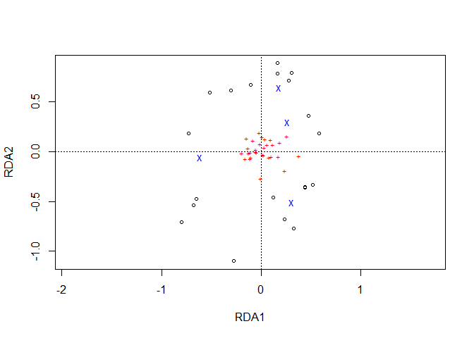
legend.key = element_blank())The ordination result needs to be plotted first via ordiplot.
plot1 <- ordiplot(Ordination.model1, choices=c(1,2))
To plot data via ggplot2, information on the locations of sites (circles in the ordiplot) is obtained via function sites.long. Information on species is extracted by function species.long.
sites.long1 <- sites.long(plot1, env.data=dune.env)
head(sites.long1)
#>    A1 Moisture Management      Use Manure     axis1      axis2 labels
#> 1 2.8        1         SF Haypastu      4 0.5831201  0.1825554      1
#> 2 3.5        1         BF Haypastu      2 0.4751761  0.3624230      2
#> 3 4.3        2         SF Haypastu      4 0.5157071 -0.3323011      3
#> 4 4.2        2         SF Haypastu      4 0.4398671 -0.3607994      4
#> 5 6.3        1         HF Hayfield      2 0.2767400  0.7134658      5
#> 6 4.3        1         HF Haypastu      2 0.1630074  0.7845782      6
Information on the labelling of the axes is obtained with function axis.long. This information is extracted from the ordination model and not the ordiplot, hence it is important to select the same axes via argument ‘choices’. The extracted information includes information on the percentage of explained variation. I suggest that you cross-check with the summary of the redundancy analysis, where information on proportion explained is given.
axis.long1 <- axis.long(Ordination.model1, choices=c(1, 2))
axis.long1
#>   axis     ggplot        label
#> 1    1 xlab.label RDA1 (16.9%)
#> 2 2 ylab.label RDA2 (9.5%)Function centroids.long obtains data on the centroids of each grouping. It is possible to directly add their results as ‘ordispider diagrams’ in ggplot. Here also another layer is added of superellipses obtained from the ggforce::geom_mark_ellipse function.
plotgg1 <- ggplot() +
    geom_vline(xintercept = c(0), color = "grey70", linetype = 2) +
    geom_hline(yintercept = c(0), color = "grey70", linetype = 2) +
    xlab(axis.long1[1, "label"]) +
    ylab(axis.long1[2, "label"]) +
    scale_x_continuous(sec.axis = dup_axis(labels=NULL, name=NULL)) +
    scale_y_continuous(sec.axis = dup_axis(labels=NULL, name=NULL)) +
    geom_mark_ellipse(data=sites.long1,
                      aes(x=axis1, y=axis2, colour=Management,
                          fill=after_scale(alpha(colour, 0.2))),
                      expand=0, size=0.2, show.legend=FALSE) +
    geom_segment(data=centroids.long(sites.long1, grouping=Management),
                 aes(x=axis1c, y=axis2c, xend=axis1, yend=axis2, colour=Management),
                 size=1, show.legend=FALSE) +
    geom_point(data=sites.long1,
               aes(x=axis1, y=axis2, colour=Management, shape=Management),
               size=5) +
    BioR.theme +
    ggsci::scale_colour_npg() +
    coord_fixed(ratio=1)

plotgg1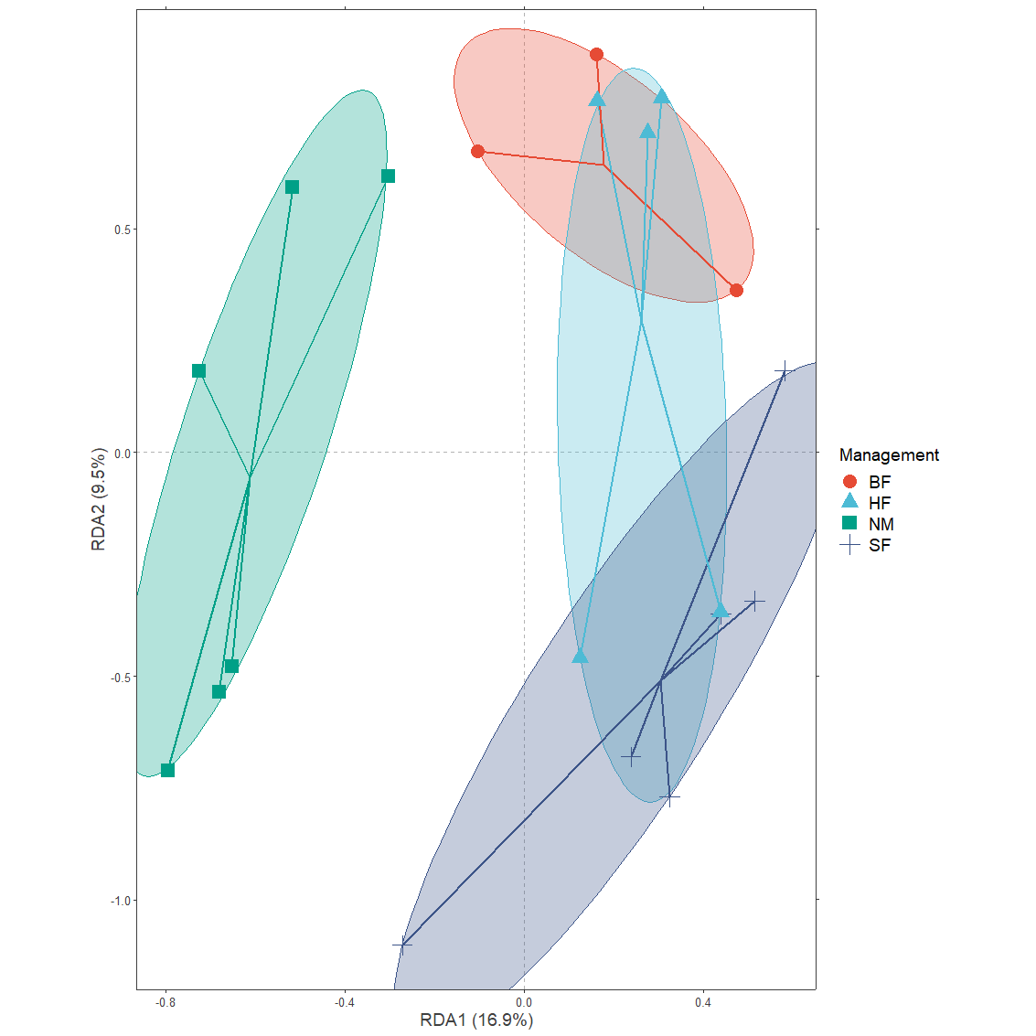
Function ordiellipse.long reproduces similar ellipses as vegan::ordiellipse.
It is necessary to re-plot the ordiplot. It is also necessary to give the name of the Management variable explicitly as this was not captured in the ordiellipse result.
plot1 <- ordiplot(Ordination.model1, choices=c(1,2))
Management.ellipses <- ordiellipse(plot1,
                                   groups=Management,
                                   display="sites",
                                   kind="sd")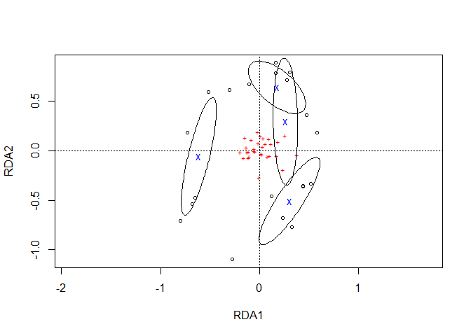
Management.ellipses.long1 <- ordiellipse.long(Management.ellipses,
grouping.name="Management")plotgg2 <- ggplot() +
geom_vline(xintercept = c(0), color = "grey70", linetype = 2) +
geom_hline(yintercept = c(0), color = "grey70", linetype = 2) +
xlab(axis.long1[1, "label"]) +
ylab(axis.long1[2, "label"]) +
scale_x_continuous(sec.axis = dup_axis(labels=NULL, name=NULL)) +
scale_y_continuous(sec.axis = dup_axis(labels=NULL, name=NULL)) +
geom_polygon(data=Management.ellipses.long1,
aes(x=axis1, y=axis2,
colour=Management,
fill=after_scale(alpha(colour, 0.2))),
size=0.2, show.legend=FALSE) +
geom_segment(data=centroids.long(sites.long1,
grouping=Management),
aes(x=axis1c, y=axis2c, xend=axis1, yend=axis2,
colour=Management),
size=1, show.legend=FALSE) +
geom_point(data=sites.long1,
aes(x=axis1, y=axis2, colour=Management, shape=Management),
size=5) +
BioR.theme +
ggsci::scale_colour_npg() +
coord_fixed(ratio=1)
plotgg2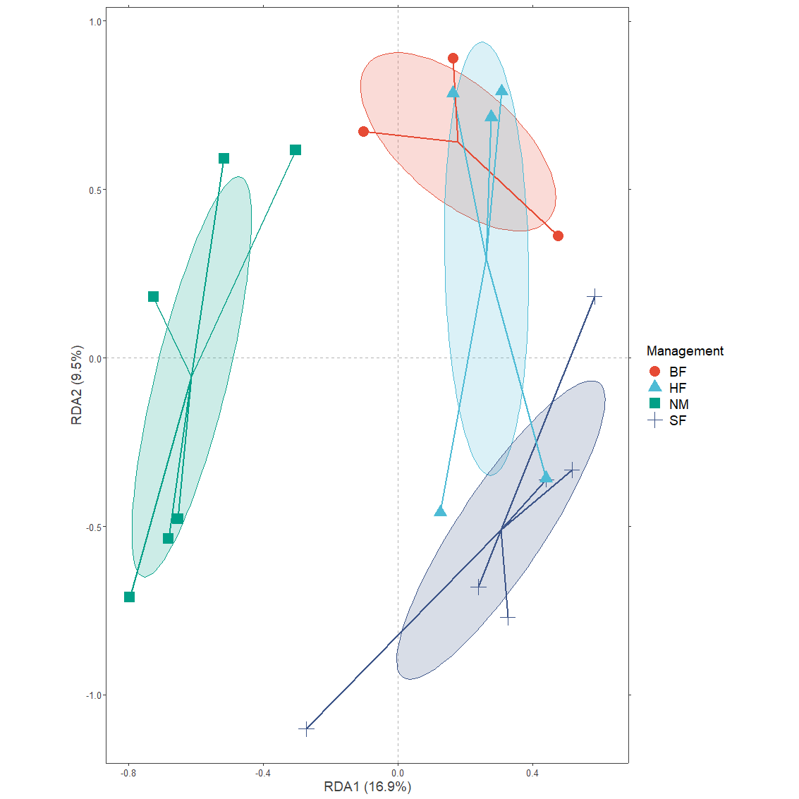
Where the previous example examined patterns for a categorical explanatory variable, here we will explore patterns for the continuous variable A1, documenting the thickness of the A1 horizon.
The vegan package includes a method of adding a smooth surface to an ordination diagram. This method is implemented in function ordisurf.
A1.surface <- ordisurf(plot1, y=A1)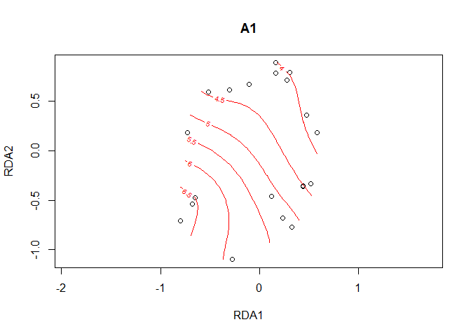
Function ordisurfgrid.long extracts the data to be plotted with ggplot2
A1.grid <- ordisurfgrid.long(A1.surface)plotgg3 <- ggplot() +
geom_contour_filled(data=A1.grid,
aes(x=x, y=y, z=z)) +
geom_vline(xintercept = c(0), color = "grey70", linetype = 2) +
geom_hline(yintercept = c(0), color = "grey70", linetype = 2) +
xlab(axis.long1[1, "label"]) +
ylab(axis.long1[2, "label"]) +
scale_x_continuous(sec.axis = dup_axis(labels=NULL, name=NULL)) +
scale_y_continuous(sec.axis = dup_axis(labels=NULL, name=NULL)) +
geom_point(data=sites.long1,
aes(x=axis1, y=axis2, shape=Management),
colour="red", size=4) +
BioR.theme +
scale_fill_viridis_d() +
labs(fill="A1") +
coord_fixed(ratio=1)
plotgg3
#> Warning: Removed 209 rows containing non-finite values (stat_contour_filled).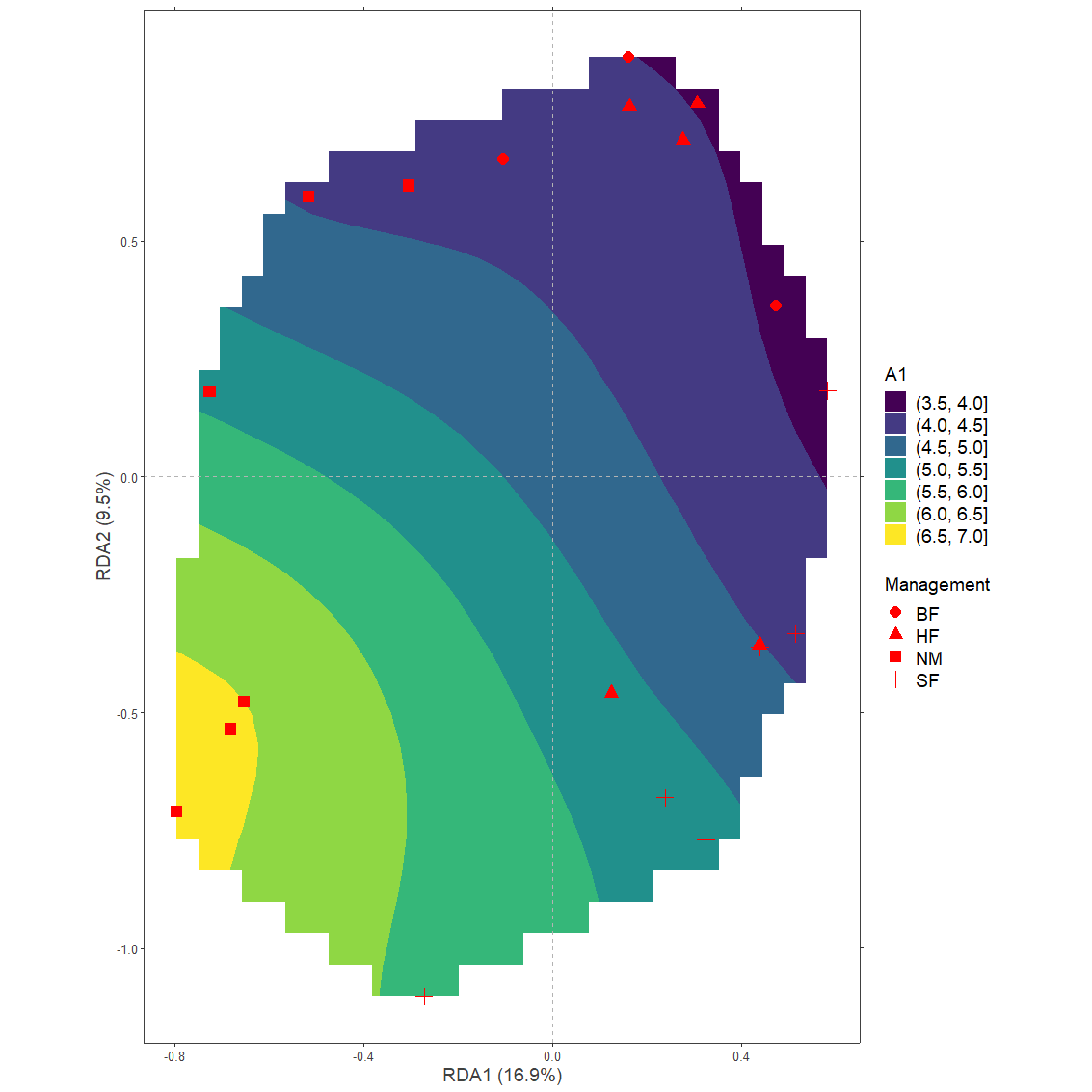
First pvclust results need to be obtained
dune.pv <- pvclust(t(dune.Hellinger),
                   method.hclust="mcquitty",
                   method.dist="euclidean",
                   nboot=1000)
#> Bootstrap (r = 0.5)... Done.
#> Bootstrap (r = 0.6)... Done.
#> Bootstrap (r = 0.7)... Done.
#> Bootstrap (r = 0.8)... Done.
#> Bootstrap (r = 0.9)... Done.
#> Bootstrap (r = 1.0)... Done.
#> Bootstrap (r = 1.1)... Done.
#> Bootstrap (r = 1.2)... Done.
#> Bootstrap (r = 1.3)... Done.
#> Bootstrap (r = 1.4)... Done.

plot(dune.pv)
pvrect(dune.pv, alpha=0.89, pv="au")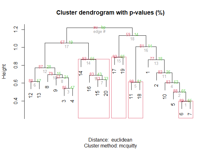
Function pvclust.long extracts the data both from the pvclust object and a ordicluster object.
plot1 <- ordiplot(Ordination.model1, choices=c(1,2), scaling='species')
cl.data1 <- ordicluster(plot1,
                        cluster=as.hclust(dune.pv$hclust))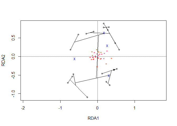
pvlong <- pvclust.long(dune.pv, cl.data1)With a similar methodology as available in ordicluster, higher clustering levels in the hierarchy can be removed via variable prune available from the results for nodes and branches.
plotgg4 <- ggplot() +
    geom_vline(xintercept = c(0), color = "grey70", linetype = 2) +
    geom_hline(yintercept = c(0), color = "grey70", linetype = 2) +
    xlab(axis.long1[1, "label"]) +
    ylab(axis.long1[2, "label"]) +
    scale_x_continuous(sec.axis = dup_axis(labels=NULL, name=NULL)) +
    scale_y_continuous(sec.axis = dup_axis(labels=NULL, name=NULL)) +
    geom_segment(data=subset(pvlong$segments,
                             pvlong$segments$prune > 3),
               aes(x=x1, y=y1, xend=x2, yend=y2,
                   colour=au>=0.89,
                   size=au),
               show.legend=TRUE) +
    geom_point(data=subset(pvlong$nodes,
                           pvlong$nodes$prune > 3),
               aes(x=x, y=y,
                   fill=au>=0.89),
               shape=21, size=2, colour="black") +
    geom_point(data=sites.long1,
               aes(x=axis1, y=axis2, shape=Management),
               colour="darkolivegreen4", alpha=0.9, size=5) +
    geom_text(data=sites.long1,
              aes(x=axis1, y=axis2, label=labels)) +
    BioR.theme +
    ggsci::scale_colour_npg() +
    scale_size(range=c(0.3, 2)) +
    scale_shape_manual(values=c(15, 16, 17, 18)) +
    guides(shape = guide_legend(override.aes = list(linetype = 0))) +
    coord_fixed(ratio=1)

plotgg4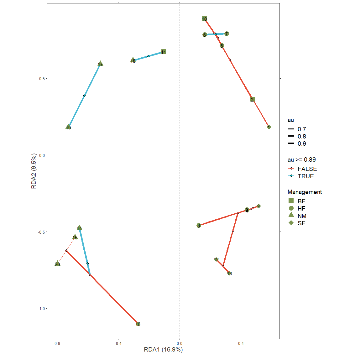
sessionInfo()
#> R version 4.0.2 (2020-06-22)
#> Platform: x86_64-w64-mingw32/x64 (64-bit)
#> Running under: Windows 10 x64 (build 19042)
#>
#> Matrix products: default
#>
#> locale:
#> [1] LC_COLLATE=English_United Kingdom.1252
#> [2] LC_CTYPE=English_United Kingdom.1252
#> [3] LC_MONETARY=English_United Kingdom.1252
#> [4] LC_NUMERIC=C
#> [5] LC_TIME=English_United Kingdom.1252
#>
#> attached base packages:
#> [1] tcltk     stats     graphics  grDevices utils     datasets  methods
#> [8] base
#>
#> other attached packages:
#>  [1] pvclust_2.2-0        dplyr_1.0.2          ggsci_2.9
#>  [4] ggrepel_0.8.2        concaveman_1.1.0     ggforce_0.3.2
#>  [7] ggplot2_3.3.3        BiodiversityR_2.14-2 vegan_2.5-6
#> [10] lattice_0.20-41      permute_0.9-5
#>
#> loaded via a namespace (and not attached):
#>  [1] nlme_3.1-148        RColorBrewer_1.1-2  tools_4.0.2
#>  [4] backports_1.1.7     R6_2.4.1            rpart_4.1-15
#>  [7] Hmisc_4.4-0         nortest_1.0-4       DBI_1.1.0
#> [10] mgcv_1.8-31         colorspace_1.4-1    nnet_7.3-14
#> [13] withr_2.2.0         tidyselect_1.1.0    gridExtra_2.3
#> [16] curl_4.3            compiler_4.0.2      htmlTable_2.0.0
#> [19] isoband_0.2.1       sandwich_2.5-1      labeling_0.3
#> [22] tcltk2_1.2-11       effects_4.1-4       scales_1.1.1
#> [25] checkmate_2.0.0     RcmdrMisc_2.7-2     stringr_1.4.0
#> [28] digest_0.6.25       foreign_0.8-80      relimp_1.0-5
#> [31] minqa_1.2.4         rmarkdown_2.3       rio_0.5.16
#> [34] base64enc_0.1-3     jpeg_0.1-8.1        pkgconfig_2.0.3
#> [37] htmltools_0.5.1.1   Rcmdr_2.7-2         lme4_1.1-23
#> [40] htmlwidgets_1.5.1   rlang_0.4.8         readxl_1.3.1
#> [43] rstudioapi_0.11     farver_2.0.3        generics_0.1.0
#> [46] zoo_1.8-8           acepack_1.4.1       zip_2.0.4
#> [49] car_3.0-8           magrittr_1.5        Formula_1.2-3
#> [52] Matrix_1.2-18       Rcpp_1.0.7          munsell_0.5.0
#> [55] abind_1.4-5         lifecycle_0.2.0     stringi_1.4.6
#> [58] yaml_2.2.1          carData_3.0-4       MASS_7.3-51.6
#> [61] grid_4.0.2          parallel_4.0.2      forcats_0.5.0
#> [64] crayon_1.3.4        haven_2.3.1         splines_4.0.2
#> [67] hms_0.5.3           knitr_1.28          pillar_1.4.4
#> [70] boot_1.3-25         glue_1.4.1          evaluate_0.14
#> [73] mitools_2.4         latticeExtra_0.6-29 data.table_1.12.8
#> [76] png_0.1-7           vctrs_0.3.4         nloptr_1.2.2.1
#> [79] tweenr_1.0.1        cellranger_1.1.0    gtable_0.3.0
#> [82] purrr_0.3.4         polyclip_1.10-0     xfun_0.15
#> [85] openxlsx_4.1.5      survey_4.0          e1071_1.7-3
#> [88] viridisLite_0.3.0   class_7.3-17        survival_3.1-12
#> [91] tibble_3.0.1        cluster_2.1.0       statmod_1.4.34
#> [94] ellipsis_0.3.1